Vlookup() function
Vlookup() function
VLOOKUP is an extremely useful tool, and learning how to use it is easier than we think!
The VLOOKUP function performs a vertical lookup by searching for a value in the first column of a table and returning the value in the same row in the index_number position. The VLOOKUP function is a built-in function in Excel that is categorized as a Lookup/Reference Function.
Syntax
There are four pieces of information that you will need in order to build the VLOOKUP syntax:
Value
|
The value you want to look up, also called the lookup value.
|
Table
|
The range where the lookup value is located. Remember that the lookup value should always be in the first column in the range for VLOOKUP to work correctly. For example, if your lookup value is in cell C2 then your range should start with C.
|
Col_index
|
The column number in the range that contains the return value. For example, if you specify B2: D11 as the range, you should count B as the first column, C as the second, and so on.
|
Range_lookup
|
Optionally, you can specify TRUE if you want an approximate match or FALSE if you want an exact match of the return value. If you don't specify anything, the default value will always be TRUE or approximate match.
|
VLOOKUP retrieves data based on column index
When you use VLOOKUP, imagine that every column in the table is numbered, starting from the left. To get a value from a particular column, simply supply the appropriate number as the "column index":
Formulae
=VLOOKUP(H3,B4:E13,2,FALSE) // first
=VLOOKUP(H3,B4:E13,3,FALSE) // last
=VLOOKUP(H3,B4:E13,4,FALSE) // email
1. H3 is lookup_value, or the value you want to look up.
2. B4 to E13 is table_array, or the range where the lookup value is located.
3. 2,3 and 4 is col_index_num, or the column number in table_array that contains the return value.
4. FALSE is range_lookup, so the return value will be an exact match.
5. Output of the VLOOKUP formula is Jonathan if the col_index_num is 2, and so on.
Example1
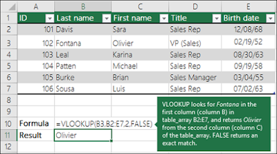
Example2
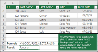
Example3
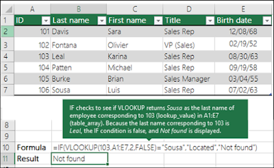
Example4
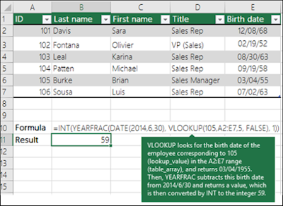
Example5
VLOOKUP has two matching modes, exact and approximate
VLOOKUP has two modes of matching: exact and approximate, which are controlled by the 4th argument, called "range_lookup". Set range_lookup to FALSE to force exact matching, and TRUE for approximate matching.
Important: range_lookup defaults to TRUE, so VLOOKUP will use approximate matching by default:
=VLOOKUP(value, table, column) // default, approximate match
=VLOOKUP(value, table, column, TRUE) // approximate match
=VLOOKUP(value, table, column, FALSE) // exact match
Example 1: Exact match
In most cases, you'll probably want to use VLOOKUP in exact match mode. This makes sense when you have a unique key to use as a lookup value, for example, the movie title in this data:
The formula in H6 to lookup year based on an exact match of movie title is:
=VLOOKUP(H4,B5:E9,2,FALSE) // FALSE = exact match
Example 2: Approximate match
You'll want to use approximate mode in cases when you're looking for the best match, not an exact match. A classic example is finding the right commission rate based on a monthly sales number. In this case, you want VLOOKUP to get you the best match for a given lookup value. In the example below, the formula in D5 performs an approximate match to retrieve the correct commission.
Your data must be sorted in ascending order by lookup value when you use approximate match mode with VLOOKUP.
Notes
· VLOOKUP supports approximate and exact matching, and wildcards (* ?) for partial matches.
· The "V" stands for "vertical".
· Lookup values must appear in the first column of the table, with lookup columns to the right.
· If you specify FALSE for the approximate_match parameter and no exact match is found, then the VLOOKUP function will return #N/A.
· If you specify TRUE for the approximate_match parameter and no exact match is found, then the next smaller value is returned.
· If col_index is less than 1, the VLOOKUP function will return #VALUE!.
· If col_index is greater than the number of columns in table, the VLOOKUP function will return #REF!
Wildcards are special characters that can take any place of any character (hence the name – wildcard). There are only 3 Excel wildcard characters (asterisk, question mark, and tilde).
The following wildcard characters can be used as comparison criteria for text filters, and when searching and replacing content.
* (asterisk)
It represents any number of characters. For example, Ex* could mean Excel, Excels, Example, Expert, etc.
? (question mark)
It represents one single character. For example, Tr?mp could mean Trump or Tramp.
~ (tilde)
It is used to identify a wildcard character (~, *, ?) in the text. For example, let’s say you want to find the exact phrase Excel* in a list. If you use Excel* as the search string, it would give you any word that has Excel at the beginning followed by any number of characters (such as Excel, Excels, Excellent). To specifically look for excel*, we need to use ~. So our search string would be excel~*. Here, the presence of ~ ensures that excel reads the following character as is, and not as a wildcard.
Filter Data using Wildcard Characters
Excel wildcard characters come in handy when you have huge data sets and you want to filter data based on a condition. Suppose you have a dataset as below. You can use the asterisk (*) wildcard character in data filter to get a list of companies that start with the alphabet A.
Here is how to do this:
1. Select the cells that you want to filter.
2. Go to Data –> Sort and Filter –> Filter (Keyboard Shortcut – Control + Shift + L).
3. Click on the filter icon in the header cell
4. In the field (below the Text Filter option), type A*
5. Click OK.
This will instantly filter the results and give you 3 names – ABC Ltd., Amazon.com, and Apple Stores.
How does it work
When you add an asterisk (*) after A, Excel would filter anything that starts with A. This is because an asterisk (being an Excel wildcard character) can represent any number of characters. Now with the same methodology, you can use various criteria to filter results.
If you use A?C instead, you will only get ABC Ltd as the result (as only one character is allowed between ‘a’ and ‘c’)
Wildcard Characters & VLOOKUP
Partial look-up is needed when you have to look for a value in a list and there isn’t an exact match. For example, suppose you have a data set as shown below, and you want to look for the company ABC in a list, but the list has ABC Ltd instead of ABC.
You cannot use the regular VLOOKUP function in this case as the lookup value does not have an exact match. If you use VLOOKUP with an approximate match, it will give you the wrong results. However, you can use a wildcard character within VLOOKUP function to get the right results:
Enter the following formula in cell D2 and drag it for other cells:
=VLOOKUP("*"&C2&"*",$A$2:$A$8,1,FALSE)
How does this formula work
In the above formula, instead of using the lookup value as is, it is flanked on both sides with the Excel wildcard character asterisk (*) – “*”&C2&”*”. This tells excel that it needs to look for any text that contains the word in C2. It could have any number of characters before or after the text in C2. Hence, the formula looks for a match, and as soon as it gets a match, it returns that value.
Find and Replace
You have data as below, the region has been entered in different ways (such as North-West, North West, NorthWest).
To clean this data and make it consistent, we can use Find and Replace with Excel wildcard characters.
Here is how to do this:
1. Select the data where you want to find and replace text.
2. Go to Home –> Find & Select –> Go To. This will open the Find and Replace dialogue box. (You can also use the keyboard shortcut – Control + H).
3. Enter the following text in the find and replace dialogue box:
4. Find what: North*W*
5. Replace with: North-West
6. Click on Replace All.
This will instantly change all the different formats and make it consistent to North-West.
How does this Work?
In the Find field, we have used North*W* which will find any text that has the word North and contains the alphabet ‘W’ anywhere after it. Hence, it covers all the scenarios (NorthWest, North West, and North-West). Find and Replace finds all these instances and changes it to North-West and makes it consistent.
IfError() Function
The Excel IFERROR function returns a custom result when a formula generates an error, and a standard result when no error is detected. IFERROR is an elegant way to trap and manage errors without using more complicated nested IF statements.
Syntax
The syntax for the IFERROR function in Microsoft Excel is:
=IFERROR( formula, alternate_value )
Parameters or Arguments
formula
The formula or value that you want to test.
value_if_error
The alternate value that is returned if the formula results in an error value (#N/A, #VALUE!, #REF!, #DIV/0!, #NUM!, #NAME? or #NULL). Otherwise, the function will return the result of the formula if no error occurs.
Excel Iferror Function Examples
Example 1
The following spreadsheet shows two simple examples of the Excel Iferror function.
Formulas:
A
|
B
|
C
| |
1
|
1
|
2
|
=IFERROR( A1 / B1, 0 )
|
2
|
1
|
0
|
=IFERROR( A2 / B2, 0 )
|
Results:
A
|
B
|
C
| ||
1
|
1
|
2
|
0.5
|
- A1 / B1 produces no error so result 0.5 is returned
|
2
|
1
|
0
|
0
|
- A2 / B2 produces an error so the alternative value 0 is returned
|
Note that:
- In the first example (in cell C1), the value argument, A1/B1 returns the value 0.5. This is not an error and so this value is returned by the Iferror function.
- In the second example (in cell C2), the value argument, A2/B2 returns the #DIV/0! error. Therefore, the Iferror function returns the value of the value_if_error argument, which is 0.
Example 2
In the following spreadsheet the Excel Iferror function is used with the Vlookup function.
If the Vlookup function successfully looks up a value, this is displayed in the cell; Otherwise, the text "not found" is displayed.
Formulas:
A
|
B
|
C
|
D
| |
1
|
Lookup List
|
Jim's Class:
|
=IFERROR( VLOOKUP( "Jim", A2:B6, 2, FALSE ), "not found" )
| |
2
|
Beth
|
Class 1
|
Mary's Class:
|
=IFERROR( VLOOKUP( "Mary", A2:B6, 2, FALSE ), "not found" )
|
3
|
Bob
|
Class 2
| ||
4
|
Alf
|
Class 2
| ||
5
|
Jim
|
Class 3
| ||
6
|
Ann
|
Class 3
| ||
Results:
A
|
B
|
C
|
D
| |
1
|
Lookup List
|
Jim's Class:
|
Class 3
| |
2
|
Beth
|
Class 1
|
Mary's Class:
|
"not found"
|
3
|
Bob
|
Class 2
| ||
4
|
Alf
|
Class 2
| ||
5
|
Jim
|
Class 3
| ||
6
|
Ann
|
Class 3
| ||
Notes:
- If formula is empty, it is evaluated as an empty string ("") and not an error.
- If value_if_error is supplied as an empty string (""), no message is displayed when an error is detected.
- If IFERROR is entered as an array formula, it returns an array of results with one item for each cell in value.


Comments
Post a Comment