INDEX MATCH with multiple criteria

So, you're an INDEX MATCH expert, using it to replace VLOOKUP entirely. But there are still a few lookups that you're not sure how to perform. Most importantly, you'd like to be able to look up a value based on multiple criteria within separate columns.

Fortunately, there is a solution. We can combine INDEX MATCH with a new tool called "array formulas" to look up a value based on multiple criteria. Here's how.

 Familiarity with INDEX MATCH is a pre-requisite for this tutorial. If you're not yet comfortable with it, check out our INDEX MATCH tutorial to get up to speed.

Defining the problem

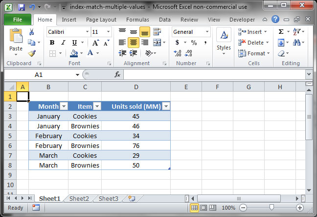
The spreadsheet below lists SnackWorld sales of both Cookies and Brownies by month. The spreadsheet is in what we call flat-file format, meaning that each separate combination of item category-month is on its own row.

We want to be able to look up the number of units sold based on a particular combination of item-month — for example, the number of Cookies sold in February.

MATCH with multiple criteria

To solve this problem, we'll have to figure out a way to use the MATCH function to match against multiple criteria columns. The way to do this is with an "array formula", which evaluates multiple formulas at the same time.

With MATCH, the easiest way to create an array formula is by using the & symbol, like so:

=MATCH(lookup_value_1&lookup_value_2, lookup_array_1&lookup_array_2, match_type)

It's very important to note that when you use an array formula like this one, you'll need to commit your formula using Ctrl+Shift+Enter rather than just pressing Enter. This will tell Excel that you're using an array formula rather than a standard formula. To show you that it's recognized an array formula, Excel will put a set of curly braces ({ }) around your entry.

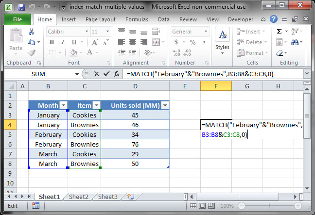
Let's take a look at an example, in which we match against two separate columns: Month and Product:

{=MATCH("February"&"Brownies",B3:B8&C3:C8, 0)}
Output: 4

In this formula, we've used the & symbol to tell MATCH to look up two criteria rather than one. Excel returns the value 4, because on the fourth row down it sees a match that satisfies both of the criteria we've provided: Column B contains the word "February" and Column C contains the word "Brownies".

Note that the order of our criteria here is important. Since our argument "February" is the first one, it's looked up within the first range provided — B3:B8. Likewise, since our "Brownies" argument comes second, it is matched in the range C3:C8.

If you're getting an error when you enter the formula, make sure you've commited with Ctrl+Shift+Enter and see those curly braces in the formula bar. Excel will give you an error if you haven't explicitly told it that you're entering an array formula.

Putting it all together

Now that we know how to use MATCH with multiple criteria, it's pretty easy to bring INDEXinto the equation. Our final formula will look something like this:

{=INDEX(range, MATCH(lookup_value_1&lookup_value_2&..., lookup_range_1&lookup_range_2&..., match_type))}

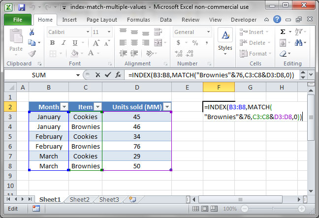
First, let's use this function to find out which month we sold 76 million units worth of Brownies:

{=INDEX(B3:B8, MATCH("Brownies"&76, C3:C8&D3:D8, 0))}
Output: "February"

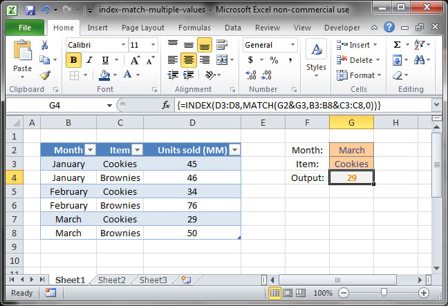
Next, let's create some dynamic input cells that let us input a month and item, then write a formula that tells Excel to pull the number of units sold for that given combination. Our INDEX MATCH formula will reference these dynamic cells with the lookup_value arguments:

{=INDEX(D3:D8, MATCH(G2&G3, B3:B8&C3:C8, 0))}
Month input: "March" (G2)
Item input: "Cookies" (G3)
Output: 29

There we have it — INDEX MATCH with multiple criteria! Note that you're not just restricted to only two criteria here, as we've done in our examples. You can add as many additional criteria as you'd like using the & symbol multiple times. Just note that performance may slow down if you chain too many of these at once in a large spreadsheet.